Introduction

A neural network is a bunch of logistic regression stacked together. A simple neural network has only one hidden layer whereas a deep neural network consists of multiple hidden layers. Every node in one layer is connected to every other node in the next layer. We make the network deeper by increasing the number of hidden layers.

This post assumes that you have a basic understanding of the intuition behind the neural network. There are so many articles on neural networks on the internet, so I won’t want to reinvent the wheel. A few of them which I found useful can be found here and here. You may wonder then why I am writing this post? When I was learning neural network I had a lot of struggle understanding the back propagation - even the online articles didn’t help much. Then I did Andrew Ng’s deep learning specialization course. I must admit he has a very simple way of explaining the most complicated concept. In this post, I will be covering backpropagation in detail. This is my attempt to give back what I learned. This post will deal with the theoretical concept, in the next post, we will apply this concept and build a homegrown neural network with Python.

Neural Network Architecture

Neural Network, like any machine learning algorithm, is a supervised learning algorithm. That means we have historic data and the corresponding label that the data maps to. The job of the neural network, like most machine learning algorithms is to find the parameters which when applied on the model will optimally fit the data. Let’s take an example of a two-layer neural network with a hidden layer of three nodes. For simplicity let’s consider the input layer with two features and a binary output. The term hidden layer refers to the fact that in the training set, the true values for these nodes in the middle are not observed. We don’t consider the input layer in the layer count. Every node on the neural network behaves like a logistic regression unit with an affine layer followed by a non-linear transformation. Essentially what each layer of the neural network does is a non-linear transformation of the input from one vector space to another. We will define items of layer-1 with superscript 1 (for eg. affine layer will be termed $Z^{[1]}$ and the activation layer as $A^{[1]}$) and layer-2 as superscript 2 ($Z^{[2]},A^{[2]}$) and so on.

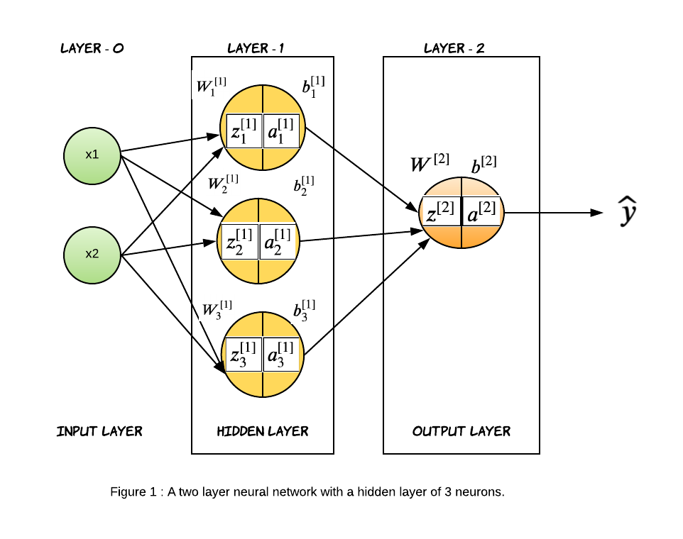
Why Neural Network? The main benefit of having a deeper model is being able to do more non-linear transformations of the input and drawing a more complex decision boundary. They are harder to debug, costlier to train but they can outperform if you have enough training data. We can fit a very complex decision boundary that generalizes pretty well.

Let’s take a closer look at what is happening in one node, then we will generalize if for the rest of the nodes. We will look at the first node of the hidden layer.

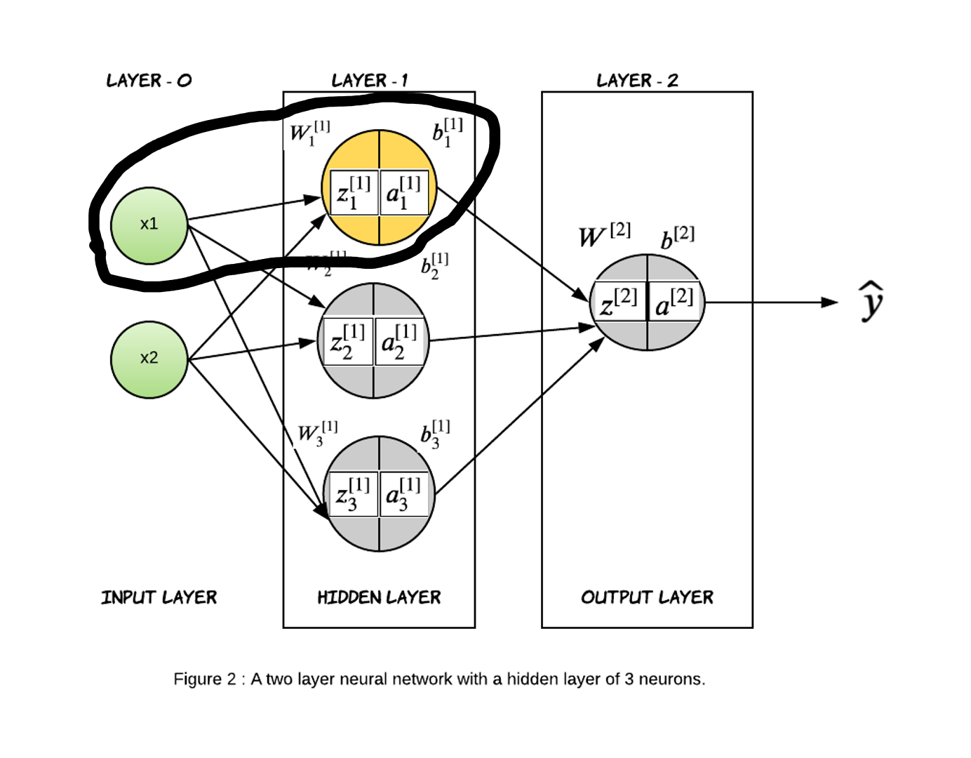
Similar to logistic regression, this node represents two steps of computation. In the first step, we will compute $z_{1}^{[1]}$ which the weighted sum of input data and parameters of the node. The second step is the activation function which is the non-linear representation. There are various activation functions one can choose from and so $g(z)$ is just a way to represent any activation function.

\[z_{1}^{[1]} = {w_{11}}^{[1]} * x_1 + {w_{12}}^{[1]} * x_2 + {b_{1}}^{[1]}\] \[a_{1}^{[1]} = g^{[1]}(z_{1}^{[1]})\]

Now, let’s represent the same equation in the vectorized form. We will consider one training example here.

\[\begin{equation} \begin{bmatrix} z_{1}^{[1]} \end{bmatrix}_{1 \times 1}= \begin{bmatrix} x_1 & x_2 \end{bmatrix}_{1 \times 2} % \begin{bmatrix} {w_{11}}^{[1]} \\ {w_{12}}^{[1]} \end{bmatrix}_{2 \times 1} + \begin{bmatrix} {b_{1}}^{[1]} \end{bmatrix}_{1 \times 1} \\\tag{1.1} \end{equation}\] \[\begin{equation} \begin{bmatrix} {a_{1}}^{[1]} \end{bmatrix}_{1 \times 1}= \begin{bmatrix} g^{[1]}({z_{1}}^{[1]}) \end{bmatrix}_{1 \times 1} \end{equation}\]

The above calculation is only for node 1 of the hidden layer(layer-1). For the rest of the nodes, we have to do a similar calculation. We can also do it all together in a vectorized form by stacking all the nodes together, which we will see in a bit. Let’s consider one single record of data for the time being. Similar to node 1, we can write node 2 and node 3 equations in the similar manner.

\[\begin{equation} \begin{bmatrix} z_{2}^{[1]} \end{bmatrix}_{1 \times 1}= \begin{bmatrix} x_1 & x_2 \end{bmatrix}_{1 \times 2} % \begin{bmatrix} {w_{21}}^{[1]} \\ {w_{22}}^{[1]} \end{bmatrix}_{2 \times 1} + \begin{bmatrix} {b_{2}}^{[1]} \end{bmatrix}_{1 \times 1} \tag{1.2} \end{equation}\] \[\begin{equation} \begin{bmatrix} {a_{2}}^{[1]} \end{bmatrix}_{1 \times 1}= \begin{bmatrix} g^{[1]}({z_{2}}^{[1]}) \end{bmatrix}_{1 \times 1} \end{equation}\] \[\begin{equation} \begin{bmatrix} z_{3}^{[1]} \end{bmatrix}_{1 \times 1}= \begin{bmatrix} x_1 & x_2 \end{bmatrix}_{1 \times 2} % \begin{bmatrix} {w_{31}}^{[1]} \\ {w_{32}}^{[1]} \end{bmatrix}_{2 \times 1} + \begin{bmatrix} {b_{3}}^{[1]} \end{bmatrix}_{1 \times 1} \tag{1.3} \end{equation}\] \[\begin{equation} \begin{bmatrix} {a_{3}}^{[1]} \end{bmatrix}_{1 \times 1}= \begin{bmatrix} g^{[1]}({z_{3}}^{[1]}) \end{bmatrix}_{1 \times 1} \end{equation}\]

Instead of calculating the nodes separately, we can combine them in one equation as follows:

\[\bbox[10px, border: 2px solid black]{ \begin{equation} \begin{bmatrix} x_1 & x_2 \end{bmatrix}_{1 \times 2} % \begin{bmatrix} {w_{11}}^{[1]} & {w_{21}}^{[1]} & {w_{31}}^{[1]} \\ {w_{12}}^{[1]} & {w_{22}}^{[1]} & {w_{32}}^{[1]} \end{bmatrix}_{2 \times 3} + \begin{bmatrix} {b_{1}}^{[1]} & {b_{2}}^{[1]} & {b_{3}}^{[1]} \end{bmatrix}_{1 \times 3} = \begin{bmatrix} z_{1}^{[1]} & z_{2}^{[1]} & z_{3}^{[1]} \end{bmatrix}_{1 \times 3} \end{equation} }\]

Basically what we did here is to stack all the weight vectors of each node as column vectors in a matrix and compute the dot product.

The output of layer-1 will be activation function applied to $Z$: \(\bbox[10px, border: 2px solid black]{ \begin{equation} \begin{bmatrix} {a_{1}}^{[1]} & {a_{2}}^{[1]} & {a_{2}}^{[1]} \end{bmatrix}_{1 \times 3}= \begin{bmatrix} g^{[1]}({z_{1}}^{[1]}) & g^{[1]}({z_{2}}^{[1]}) & g^{[1]}({z_{3}}^{[1]}) \end{bmatrix}_{1 \times 3} \end{equation} }\)

Now that we have successfully calculated the output of layer 1, let’s take a closer look at layer-2, which also happens to be the output layer in our case.

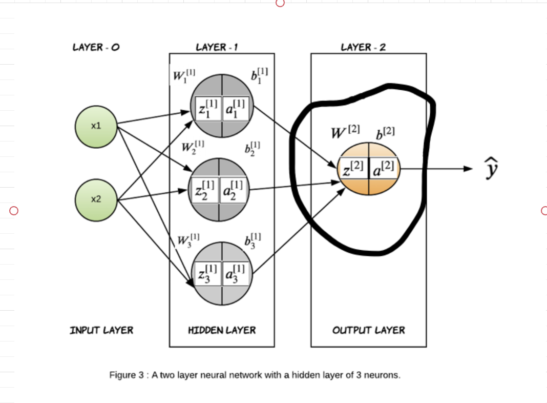
The input to the layer-2 will be the activation output of layer-1 and since it is the output layer with binary classification, we will use sigmoid as the activation function. \(\bbox[10px, border: 2px solid black]{ \begin{equation} \begin{bmatrix} z^{[2]} \end{bmatrix}_{1 \times 1}= \begin{bmatrix} {a_{1}}^{[1]} & {a_{2}}^{[1]} & {a_{3}}^{[1]} \end{bmatrix}_{1 \times 3} %tivation \begin{bmatrix} {w_{1}}^{[2]} \\ {w_{2}}^{[2]} \\ {w_{3}}^{[2]} \end{bmatrix}_{3 \times 1} + b^{[2]} \end{equation} }\)

\[\bbox[10px, border: 2px solid black]{ \begin{equation} \begin{bmatrix} {a}^{[2]} \end{bmatrix}_{1 \times 1}= \begin{bmatrix} \sigma({z}^{[2]}) \end{bmatrix}_{1 \times 1} = \widehat{y} \end{equation} }\]

If you look closely at the weight matrix, you will notice the size of the weight matrix for layer $l$ is the number of nodes of the layer $(l-1)$ by the number of nodes of layer $l$. For the input layer, consider the number of features as the number of nodes.

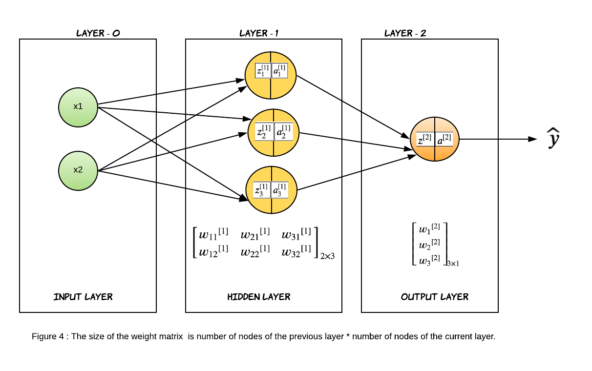
Vectorized Representation of Neural Network

In a typical machine learning problem, we will have a multitude of data. If we have a dataset of m records with n feature each, the matrix-vector representation of the Layer-1 will look like this:

\[\begin{equation} \begin{bmatrix} {z_{11}}^{[1]} & {z_{21}}^{[1]} & {z_{31}}^{[1]}\\ {z_{12}}^{[1]} & {z_{22}}^{[1]} & {z_{32}}^{[1]}\\ {z_{13}}^{[1]} & {z_{23}}^{[1]} & {z_{33}}^{[1]}\\ \vdots \\ {z_{1m}}^{[1]} & {z_{2m}}^{[1]} & {z_{3m}}^{[1]} \end{bmatrix}_{ m \times 3}= \begin{bmatrix} x_{11} & x_{12} & x_{13} & ... & x_{1n} \\ x_{21} & x_{22} & x_{23} & ... & x_{2n} \\ x_{31} & x_{32} & x_{33} & ... & x_{3n} \\ \vdots \\ x_{m1} & x_{m2} & x_{m3} & ... & x_{mn} \\ \end{bmatrix}_{ m \times n} % \begin{bmatrix} {w_{11}}^{[1]} & {w_{21}}^{[1]} & {w_{31}}^{[1]}\\ {w_{12}}^{[1]} & {w_{22}}^{[1]} & {w_{32}}^{[1]}\\ {w_{13}}^{[1]} & {w_{23}}^{[1]} & {w_{33}}^{[1]}\\ \vdots \\ {w_{1n}}^{[1]} & {w_{2n}}^{[1]} & {w_{3n}}^{[1]}\\ \end{bmatrix}_{ n\times 3} + \begin{bmatrix} {b_{1}}^{[1]} & {b_{2}}^{[1]} & {b_{3}}^{[1]} \end{bmatrix} \end{equation}\] \[\begin{equation} \begin{bmatrix} {a_{11}}^{[1]} & {a_{21}}^{[1]} & {a_{31}}^{[1]}\\ {a_{12}}^{[1]} & {a_{22}}^{[1]} & {a_{32}}^{[1]}\\ {a_{13}}^{[1]} & {a_{23}}^{[1]} & {a_{33}}^{[1]}\\ \vdots \\ {a_{1m}}^{[1]} & {a_{2m}}^{[1]} & {a_{3m}}^{[1]} \end{bmatrix}_{ m \times 3}= \begin{bmatrix} g^{[1]}({z_{11}}^{[1]}) & g^{[1]}({z_{21}}^{[1]}) & g^{[1]}({z_{31}}^{[1]})\\ g^{[1]}({z_{12}}^{[1]}) & g^{[1]}({z_{22}}^{[1]}) & g^{[1]}({z_{32}}^{[1]})\\ g^{[1]}({z_{13}}^{[1]}) & g^{[1]}({z_{23}}^{[1]}) & g^{[1]}({z_{33}}^{[1]})\\ \vdots \\ g^{[1]}({z_{1m}}^{[1]}) & g^{[1]}({z_{2m}}^{[1]}) & g^{[1]}({z_{3m}}^{[1]}) \end{bmatrix}_{ m \times 3} \end{equation}\]

The above two equations can be generalized as : \(Z^{[1]} = X \cdot W^{[1]} + b^{[1]}\)

\[A^{[1]} = g^{[1]}(Z^{[1]})\]

Similarly, for Layer-2 which is the output layer in our case, the matrix-vector representation will look like the following for m records. Remember since this is the binary classification problem we will use sigmoid as the activation layer.

\[\begin{equation} \begin{bmatrix} {z_{1}}^{[2]} \\ {z_{2}}^{[2]} \\ {z_{3}}^{[2]} \\ \vdots \\ {z_{m}}^{[2]} \end{bmatrix}_{m \times 1}= \begin{bmatrix} {a_{11}}^{[1]} & {a_{21}}^{[1]} & {a_{31}}^{[1]}\\ {a_{12}}^{[1]} & {a_{22}}^{[1]} & {a_{32}}^{[1]}\\ {a_{13}}^{[1]} & {a_{23}}^{[1]} & {a_{33}}^{[1]}\\ \vdots \\ {a_{1m}}^{[1]} & {a_{2m}}^{[1]} & {a_{3m}}^{[1]} \end{bmatrix}_{ m \times 3} % \begin{bmatrix} {w_{1}}^{[2]} \\ {w_{2}}^{[2]} \\ {w_{3}}^{[2]} \end{bmatrix}_{3 \times 1} + b^{[2]} \end{equation}\] \[\begin{equation} \begin{bmatrix} {a_{1}}^{[2]} \\ {a_{2}}^{[2]} \\ {a_{3}}^{[2]} \\ \vdots \\ {a_{m}}^{[2]} \end{bmatrix}_{m \times 1}= \begin{bmatrix} \sigma{({z_{1}}^{[2]})} \\ \sigma{({z_{2}}^{[2]})} \\ \sigma{({z_{3}}^{[2]})} \\ \vdots \\ \sigma{({z_{m}}^{[2]})} \end{bmatrix}_{m \times 1} \end{equation}\]

The above two equations can be generalized as : \(Z^{[2]} = A^{[1]} \cdot W^{[2]} + b^{[2]}\)

\[A^{[2]} = g^{[2]}(Z^{[2]})\]

Considering $X$ as Layer-0, $X$ can be represented as $A^{[0]}$. And now you can generalize the equations for Layer-l as :

\[\large \bbox[10px, border: 2px solid black]{ Z^{[l]} = A^{[l-1]} \cdot W^{[1]} + b^{[1]} }\]

\[\large \bbox[10px, border: 2px solid black]{ A^{[l]} = g^{[l]}(Z^{[l]}) }\]

The Gradient Descent Algorithm

So far we have described the forward pass, meaning given an input and weights how the output is computed. After the training is complete, we only run the forward pass to make the predictions. But we first need to train our model to actually learn the weights, and the training procedure works as follows:

• 1. Randomly initialize the weights for all the nodes.
• Loop :
  • 1. For every training example, perform a forward pass using the current weights, and calculate the output of each node going from left to right. The final output is the value of the last node.
  • 1. Compare the final output with the actual target in the training data, and measure the error using a loss function.
  • 1. Perform a backward pass from right to left and propagate the error to every individual node using backpropagation.
  • 1. Calculate each weight’s contribution to the error, and adjust the weights accordingly using gradient descent.

The weights should be randomly initialized and not set to zero initially. Otherwise each node in the hidden layer will perform the same computation. So, even after multiple iterations of gradient descent, each neuron in the layer will be computing the same thing as other neurons which will not add value.

Just like Logistic Regression, we use the log loss or cross-entropy loss as the cost function for the neural network classification problem.

\[\large loss = - y \cdot \log(\widehat{y}) - (1-y) \cdot log(1-\widehat{y})\]

The above equation is only for one training example. For a training sample of m records, the cost function can be defined as :

\[\bbox[10px, border: 2px solid black]{\large J(W,b) = \frac{1}{m} \displaystyle\sum_{i=1}^{m} -y_i \cdot \log(\widehat{y_i}) - (1-y_i) \cdot log(1-\widehat{y_i})}\]

The Backward Propagation

Let’s go back to our original example and see how far we have come. If you remember we started with a 2-layer neural network with an input of two features. The hidden layer had three nodes and the output layer had one node as it was a binary classification problem. We have initialized the weights and did a forward propagation. We have also defined our loss function. Now, we will do the backward propagation for one training example and then generalize for a dataset of m records. Here are the equations we have computed so far.

\[\begin{equation} \begin{bmatrix} z_{1}^{[1]} & z_{2}^{[1]} & z_{3}^{[1]} \end{bmatrix}_{1 \times 3} = \begin{bmatrix} x_1 & x_2 \end{bmatrix}_{1 \times 2} % \begin{bmatrix} {w_{11}}^{[1]} & {w_{21}}^{[1]} & {w_{31}}^{[1]} \\ {w_{12}}^{[1]} & {w_{22}}^{[1]} & {w_{32}}^{[1]} \end{bmatrix}_{2 \times 3} + \begin{bmatrix} {b_{1}}^{[1]} & {b_{2}}^{[1]} & {b_{3}}^{[1]} \end{bmatrix}_{1 \times 3} \tag 1 \end{equation}\] \[\begin{equation} \begin{bmatrix} {a_{1}}^{[1]} & {a_{2}}^{[1]} & {a_{2}}^{[1]} \end{bmatrix}_{1 \times 3}= \begin{bmatrix} g^{[1]}({z_{1}}^{[1]}) & g^{[1]}({z_{2}}^{[1]}) & g^{[1]}({z_{3}}^{[1]}) \end{bmatrix}_{1 \times 3} \tag 2 \end{equation}\] \[\begin{equation} \begin{bmatrix} z^{[2]} \end{bmatrix}_{1 \times 1}= \begin{bmatrix} {a_{1}}^{[1]} & {a_{2}}^{[1]} & {a_{3}}^{[1]} \end{bmatrix}_{1 \times 3} %tivation \begin{bmatrix} {w_{1}}^{[2]} \\ {w_{2}}^{[2]} \\ {w_{3}}^{[2]} \end{bmatrix}_{3 \times 1} + b^{[2]} \tag 3 \end{equation}\] \[\begin{equation} \begin{bmatrix} {a}^{[2]} \end{bmatrix}_{1 \times 1}= \begin{bmatrix} \sigma({z}^{[2]}) \end{bmatrix}_{1 \times 1} = \widehat{y} \tag 4 \end{equation}\]

Our main objective is to differentiate the loss function with respect to the parameters ($W^{[1]},b^{[1]},W^{[2]},b^{[2]}$) so that we can update the parameters with the gradients. We will see how to update the parameters in the next section, but for now, we are interested in calculating $\large \frac{\partial loss}{\partial W^{[2]}},\frac{\partial loss}{\partial b^{[2]}},\frac{\partial loss}{\partial W^{[1]}},\frac{\partial loss}{\partial b^{[1]}}.$

However, there is no easy way to calculate gradients. We have to fall back on the chain rule to derive the gradients. The red arrows in the above figure (Figure 5) depict the path the loss has to propagate to calculate the gradients of layer-1. Similarly, the blue arrows depict the path the loss has to propagate to calculate the gradients of layer-2. Since we are working on a 2-layer network, the output of the second layer is the predicted output which is $a^{[2]}$ in our case. We calculate the loss on the predicted output $a^{[2]}$. In the backward propagation, we always start from the loss and move to the left. That means we will calculate the gradients of layer-2 first and then move to layer-1.

• Gradients of Layer-2

With the help of chain rule let’s see how the gradients of the parameters of layer -2 will look like: \(\large \frac{\partial loss}{\partial W^{[2]}}= \frac{\partial loss}{\partial a^{[2]}} \times \frac{\partial a^{[2]}}{\partial z^{[2]}} \times \frac{\partial z^{[2]}}{\partial W^{[2]}}\)

\[\large \frac{\partial loss}{\partial b^{[2]}}= \frac{\partial loss}{\partial a^{[2]}} \times \frac{\partial a^{[2]}}{\partial z^{[2]}} \times \frac{\partial z^{[2]}}{\partial b^{[2]}}\]

It might look daunting at first, but don’t worry- we will attack each of them separately. Let’s start of finding the gradient of the loss w.r.t $a^{[2]}$.

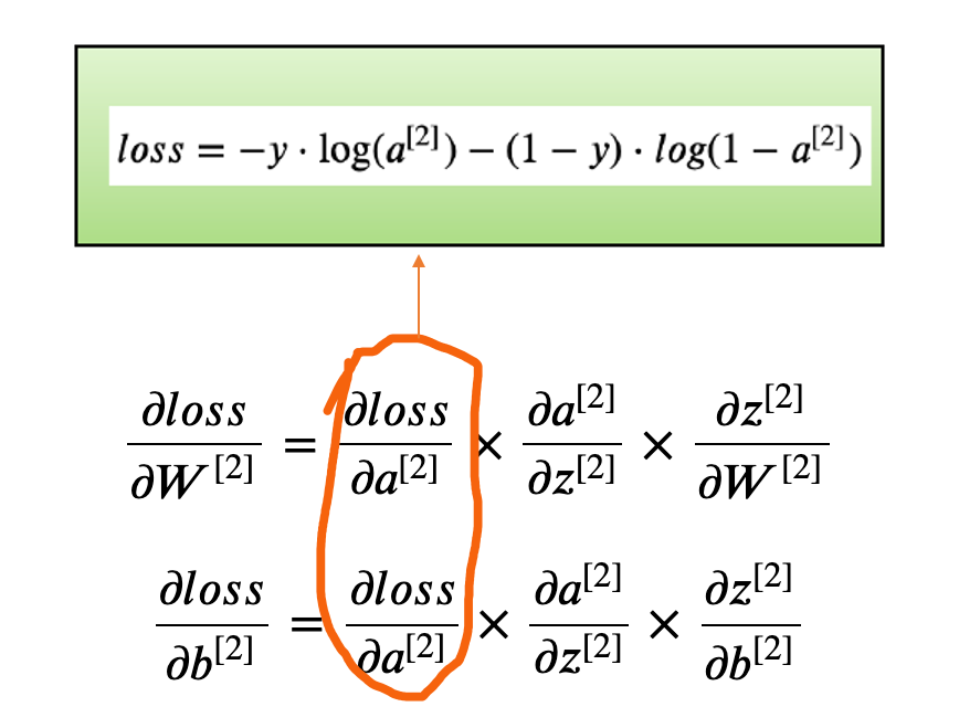
Starting with the loss function, let’s calculate the gradient w.r.t $a^{[2]}$

\[loss = - y \cdot \log(a^{[2]}) - (1-y) \cdot log(1-a^{[2]})\]

\(\frac{\partial loss}{\partial a^{[2]}}= - \frac{y}{a^{[2]}} - \frac {1-y}{1-a^{[2]}} \cdot (-1)\) Remember that there is an additional ($-1$) in the last term when we take the derivative of $(1-a^{[2]})$ with respect to $a^{[2]}$ (remember the Chain Rule). After cleaning up the terms, the equation becomes:

\[\frac{\partial loss}{\partial a^{[2]}}= \frac{-y}{a^{[2]}} + \frac{1-y}{1-a^{[2]}} = \frac {(a^{[2]} - y)}{a^{[2]} (1- a^{[2]})}\]

Now, let’s attack the next derivative term.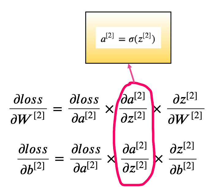

This the activation layer of the Layer-2, which has a sigmoid activation function. The derivative of a sigmoid has the form:

\[\frac{d}{dz}\sigma(z) = \sigma(z) \times (1 - \sigma(z))\]

Recall that $\sigma(z) = a^{[2]} $, because we defined “$a^{[2]} $”, the activation, as the output of the sigmoid activation function.

So we can substitute into the formula to get:

\[\frac{\partial a^{[2]}}{\partial z^{[2]}} = a^{[2]} (1 - a^{[2]})\]

Now, if we combine the two gradients, the equation gets much more simplified.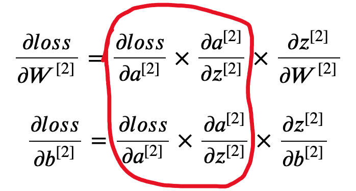

\[\large \frac{\partial loss}{\partial z^{[2]}} = {(a^{[2]} - y)}\]

So far so good, now let’s look at the last part of the gradients.

\[\frac{\partial z^{[2]}}{\partial W^{[2]}} = a^{[1]}\] \[\frac{\partial z^{[2]}}{\partial b^{[2]}} = 1\]

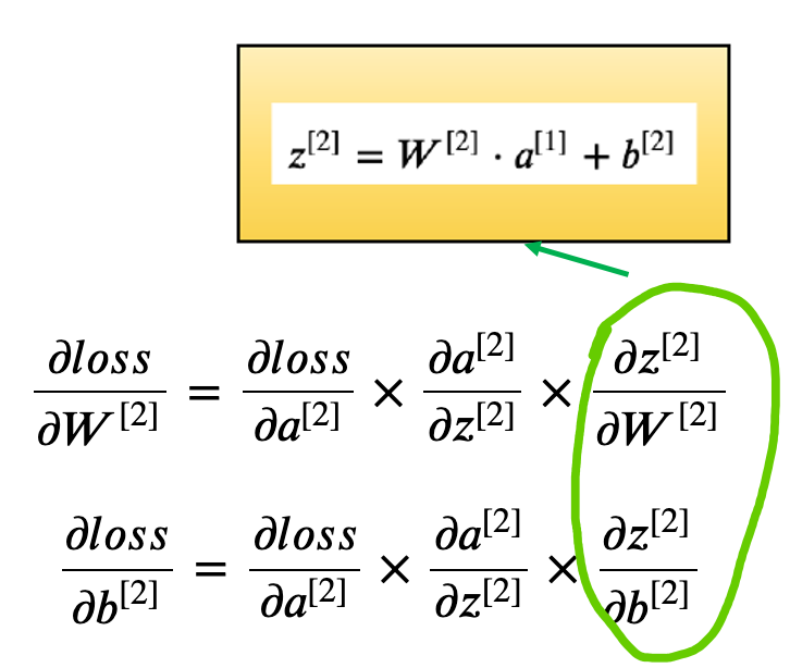
Now, let’s combine the gradients. \(\frac{\partial loss}{\partial W^{[2]}}= \frac{\partial loss}{\partial a^{[2]}} \times \frac{\partial a^{[2]}}{\partial z^{[2]}} \times \frac{\partial z^{[2]}}{\partial W^{[2]}}=\frac{\partial loss}{\partial z^{[2]}} \times \frac{\partial z^{[2]}}{\partial W^{[2]}} = (a^{[1]})^{T} \cdot (a^{[2]} - y)\)

\[\frac{\partial loss}{\partial b^{[2]}}= \frac{\partial loss}{\partial a^{[2]}} \times \frac{\partial a^{[2]}}{\partial z^{[2]}} \times \frac{\partial z^{[2]}}{\partial b^{[2]}}=\frac{\partial loss}{\partial z^{[2]}} \times \frac{\partial z^{[2]}}{\partial W^{[2]}} = 1\cdot (a^{[2]} - y)\]

Note: You may need to transpose the matrix /vector sometimes so as to match up the dimensions required to do a dot product.

\[\frac{\partial loss}{\partial W^{[2]}}= \begin{equation} \begin{bmatrix} {a_{1}}^{[1]} \\ {a_{2}}^{[1]} \\ {a_{3}}^{[1]} \end{bmatrix}_{3 \times 1} % \begin{bmatrix} a^{[2]}-y \end{bmatrix}_{1 \times 1} = \begin{bmatrix} {a_{1}}^{[1]} (a^{[2]}-y) \\ {a_{2}}^{[1]} (a^{[2])}-y) \\ {a_{3}}^{[1]} (a^{[2])}-y) \end{bmatrix}_{3 \times 1} \end{equation}\] \[\frac{\partial loss}{\partial b^{[2]}}= \begin{equation} \begin{bmatrix} a^{[2]}-y \end{bmatrix}_{1 \times 1} \end{equation}\]

Always remember the dimensions of the gradients should always match the original dimensions.

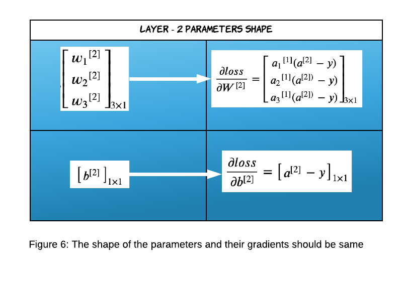
We did the above calculation on only one training example. If we have a dataset of m records then the cost function will look like this: \(J(W,b) = \frac{1}{m} \displaystyle\sum_{i=1}^{m} -y_i \cdot \log(\widehat{y}) - (1-y_i) \cdot log(1-\widehat{y})\)

The cost function finds the average loss of all the training examples and hence that is carried forward to the gradients too. The summation sign is not present in the gradient calculation of $W^{[2]}$ because the dot product does the summation internally. Finally, the gradients of Layer-2 look like below.

\[\bbox[10px, border: 2px solid black]{\large \frac{\partial loss}{\partial W^{[2]}}= \frac{1}{m} (a^{[1]})^{T} \cdot (a^{[2]} - y)}\] \[\bbox[10px, border: 2px solid black]{\large \frac{\partial loss}{\partial b^{[2]}} =\frac{1}{m} \displaystyle\sum_{i=1}^{m}(a^{[2]} - y)}\]

• Gradients of Layer-1

We are done with Layer-2, now let’s move on to Layer-1. We will follow the red line to calculate the gradients of layer-1.

\[\large \frac{\partial loss}{\partial W^{[1]}}= \frac{\partial loss}{\partial a^{[2]}} \times \frac{\partial a^{[2]}}{\partial z^{[2]}} \times \frac{\partial z^{[2]}}{\partial a^{[1]}}\times \frac{\partial a^{[1]}}{\partial z^{[1]}}\times \frac{\partial z^{[1]}}{\partial W^{[1]}}\] \[\large \frac{\partial loss}{\partial b^{[1]}}= \frac{\partial loss}{\partial a^{[2]}} \times \frac{\partial a^{[2]}}{\partial z^{[2]}} \times \frac{\partial z^{[2]}}{\partial a^{[1]}}\times \frac{\partial a^{[1]}}{\partial z^{[1]}}\times \frac{\partial z^{[1]}}{\partial b^{[1]}}\]

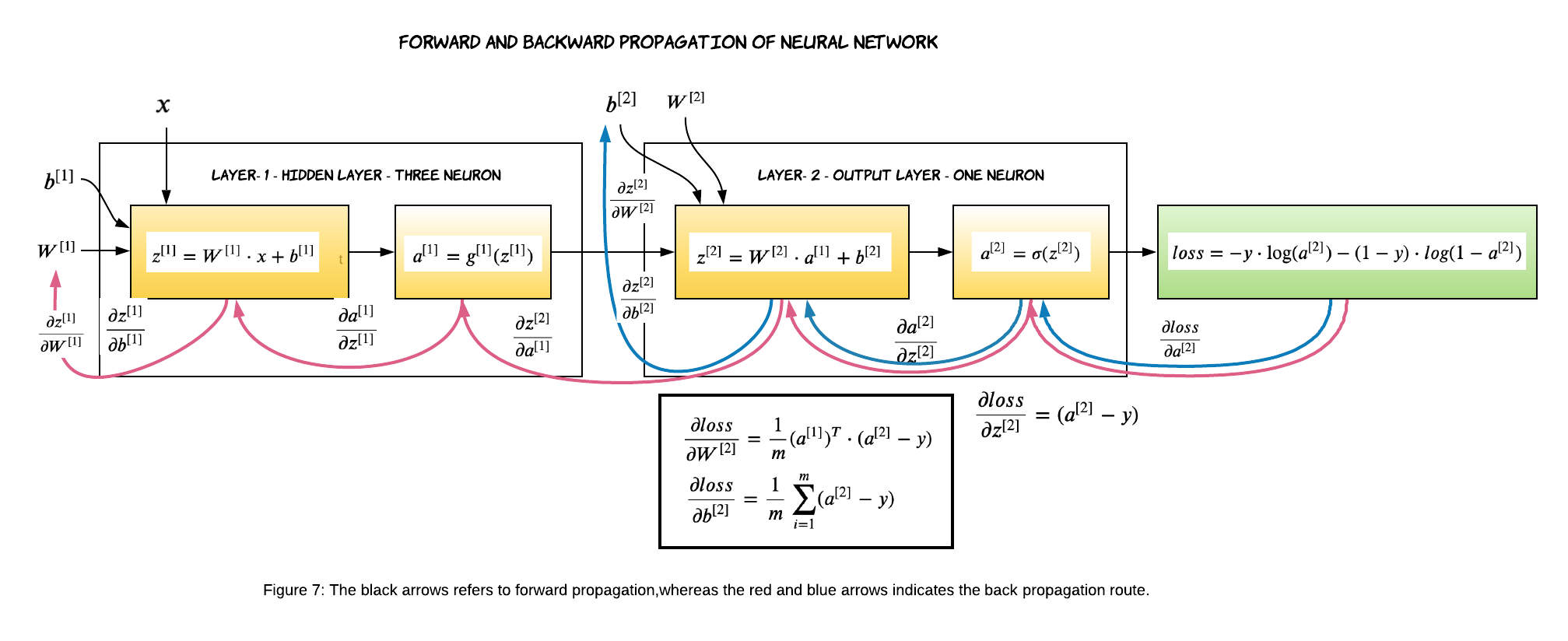
Parts of the gradients that are coming from Layer-2 has already been calculated. So, We only need to calculate the ones specific to Layer-1.

\[\frac{\partial z^{[2]}}{\partial a^{[1]}} = W^{[2]}\]

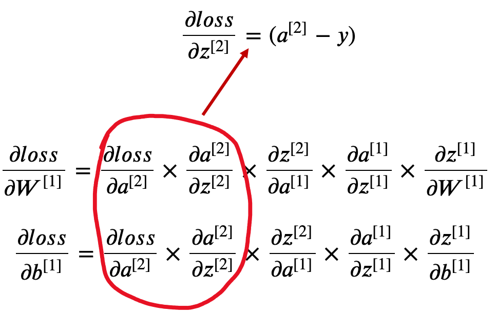
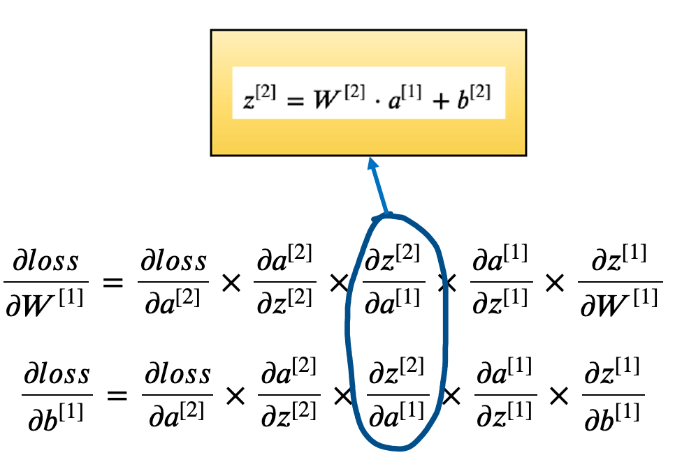
Now, if we combine the three gradients, we will get the derivative of loss w.r.t $a^{[1]}$.

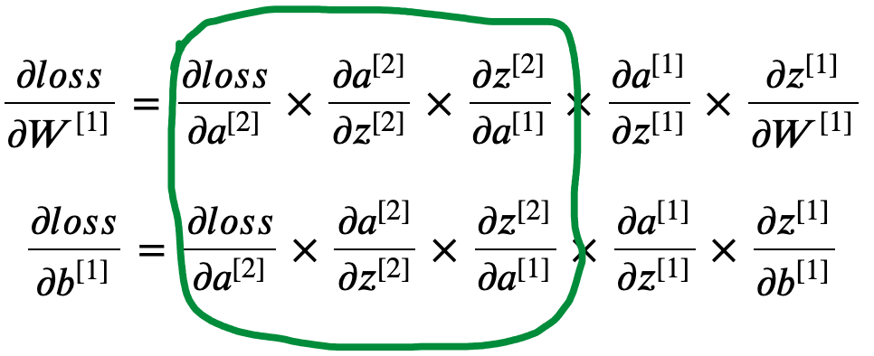
As I mentioned before, one way to find out if the calculations are correct to make sure the shape of the parameter and it’s gradients are the same. And sometimes, you have to transpose a vector or matrix to make it happen. Before we go further let’s see if $\frac{\partial loss}{\partial a^{[1]}}$ match with the size of $a^{[1]}$.

\[\frac{\partial loss}{\partial a^{[1]}}= \frac{\partial loss}{\partial a^{[2]}} \times \frac{\partial a^{[2]}}{\partial z^{[2]}} \times \frac{\partial z^{[2]}}{\partial a^{[1]}} = (a^{[2]} - y)\cdot {W^{[2]}}^T\]

$a^{[1]}$ was a 1 by 3 dimensional vector and by transposing $W^{[2]}$, we achieved the same dimension for its gradient.

\[\frac{\partial loss}{\partial a^{[1]}}= \begin{equation} \begin{bmatrix} a^{[2]}-y \end{bmatrix}_{1 \times 1} % \begin{bmatrix} {w_{1}}^{[2]} & {w_{2}}^{[2]} & {w_{3}}^{[2]} \end{bmatrix}_{1 \times 3} = \begin{bmatrix} (a^{[2]}-y){w_{1}}^{[2]} & (a^{[2])}-y){w_{2}}^{[2]} & (a^{[2])}-y){w_{3}}^{[2]} \end{bmatrix}_{1 \times 3} \end{equation}\]

Let’s move to the next item where we will calculate the gradient of $a^{[1]}$ w.r.t $z^{[1]}$. This is the activation layer of Layer-1. Since we can use any activation(tanh, relu, sigmoid etc.) in the hidden layers, we will keep this generic. Whatever activation function we have chosen in the hidden layer, we just have to find the gradient of that activation function.

\[\frac{\partial a^{[1]}}{\partial z^{[1]}} = {g^{[1]}}^{\prime}(z^{[1]})\]

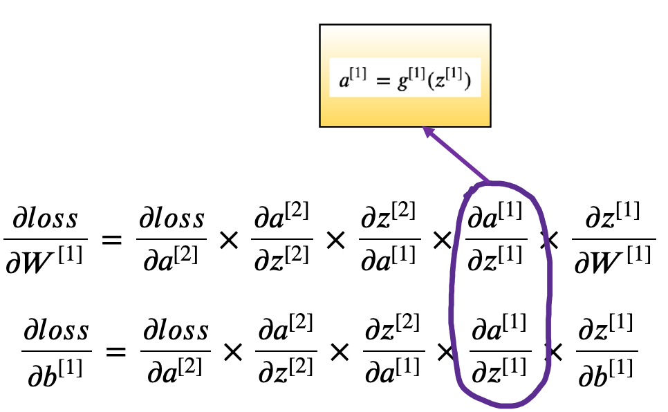
During forward propagation, you might have noticed that applying activation doesn’t change the dimension of the matrix. Activation is applied to each element of the matrix. The same holds true for it’s derivative too. This is just a multiplication step and not a dot product.

\[\begin{equation} \frac{\partial loss}{\partial z^{[1]}}= \frac{\partial loss}{\partial a^{[1]}} \times \frac{\partial a^{[1]}}{\partial z^{[1]}} = (a^{[2]} - y)\cdot {W^{[2]}}^T * {g^{[1]}}^{\prime}(z^{[1]}) = \begin{bmatrix} (a^{[2]}-y){w_{1}}^{[2]}* {g^{[1]}}^{\prime}(z^{[1]}) & (a^{[2])}-y){w_{2}}^{[2]}* {g^{[1]}}^{\prime}(z^{[1]}) & (a^{[2])}-y){w_{3}}^{[2]}* {g^{[1]}}^{\prime}(z^{[1]}) \end{bmatrix}_{1 \times 3} \end{equation}\]

We are very close, let’s find the derivative of the last chain.

\[\frac{\partial z^{[1]}}{\partial W^{[1]}}= x\] \[\frac{\partial z^{[1]}}{\partial b^{[1]}}= 1\]

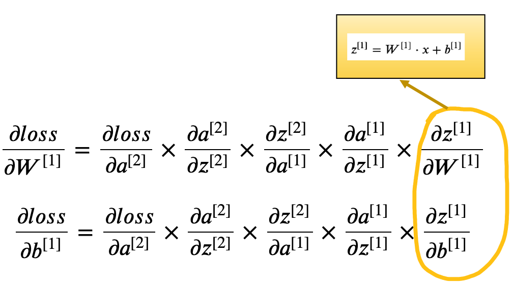
All together we get:

\[\frac{\partial loss}{\partial W^{[1]}}=\frac{\partial loss}{\partial z^{[1]}} \times \frac{\partial z^{[1]}}{\partial W^{[1]}}= x^{T} \cdot (a^{[2]} - y)\cdot {W^{[2]}}^T * {g^{[1]}}^{\prime}(z^{[1]})\] \[\frac{\partial loss}{\partial b^{[1]}}=\frac{\partial loss}{\partial z^{[1]}} \times \frac{\partial z^{[1]}}{\partial b^{[1]}}= (a^{[2]} - y)\cdot {W^{[2]}}^T * {g^{[1]}}^{\prime}(z^{[1]})\]

Like we did for Layer-2, we will check if the dimensions of the $W^{[1]}$ and $b^{[1]}$ are same as their gradients.

\[\frac{\partial loss}{\partial W^{[1]}}= x^{T} \cdot \frac{\partial loss}{\partial z^{[1]}}\] \[\begin{equation} \begin{bmatrix} x_1 \\ x_2 \end{bmatrix}_{2 \times 1} \cdot % \begin{bmatrix} (a^{[2]}-y){w_{1}}^{[2]}* {g^{[1]}}^{\prime}(z^{[1]}) & (a^{[2])}-y){w_{2}}^{[2]}* {g^{[1]}}^{\prime}(z^{[1]}) & (a^{[2])}-y){w_{3}}^{[2]}* {g^{[1]}}^{\prime}(z^{[1]}) \end{bmatrix}_{1 \times 3} = % \begin{bmatrix} x_1 * (a^{[2]}-y){w_{1}}^{[2]}* {g^{[1]}}^{\prime}(z^{[1]}) & x_1 * (a^{[2])}-y){w_{2}}^{[2]}* {g^{[1]}}^{\prime}(z^{[1]}) & x_1 * (a^{[2])}-y){w_{3}}^{[2]}* {g^{[1]}}^{\prime}(z^{[1]}) \\ x_2 * (a^{[2]}-y){w_{1}}^{[2]}* {g^{[1]}}^{\prime}(z^{[1]}) & x_2 * (a^{[2])}-y){w_{2}}^{[2]}* {g^{[1]}}^{\prime}(z^{[1]}) & x_2 * (a^{[2])}-y){w_{3}}^{[2]}* {g^{[1]}}^{\prime}(z^{[1]}) \end{bmatrix}_{2 \times 3} \end{equation}\]

It is a very complication equation and I know it’s very difficult to follow along but I just want to prove that the dimension of the gradient is 2 $\times$ 3 and is same as the original weight dimension.

Oh, one last thing, as mentioned earlier while calculating gradient for a dataset of m records we have to have a summation and a division by m (carry forward from the loss function).

\[\large \bbox[10px, border: 2px solid black]{\frac{\partial loss}{\partial W^{[1]}}= \frac{1}{m}x^{T} \cdot (a^{[2]} - y)\cdot {W^{[2]}}^T * {g^{[1]}}^{\prime}(z^{[1]})}\] \[\large \bbox[10px, border: 2px solid black]{\frac{\partial loss}{\partial b^{[1]}} = \frac{1}{m} \displaystyle\sum_{i=1}^{m} (a^{[2]} - y)\cdot {W^{[2]}}^T * {g^{[1]}}^{\prime}(z^{[1]})}\]

Update Parameters

In the final step, we use the gradients to update the parameters. There is still another parameter to consider: the learning rate, denoted by the Greek letter eta (that looks like the letter n), which is the multiplicative factor that we need to apply to the gradient for the parameter update. The learning rate is a tuning parameter in an optimization algorithm that determines the step size at each iteration while moving toward a minimum of a loss function.

\[W^{[2]} := W^{[2]} - \eta \frac{\partial loss}{\partial W^{[2]}}\] \[b^{[2]} := b^{[2]} - \eta \frac{\partial loss}{\partial b^{[2]}}\] \[W^{[1]} := W^{[1]} - \eta \frac{\partial loss}{\partial W^{[1]}}\] \[b^{[1]} := b^{[1]} - \eta \frac{\partial loss}{\partial b^{[1]}}\]

Conclusion

In this article we took an example of a shallow neural network and did a forward propagation, then computed the loss function and went through the math behind the backward propagation in details. I hope you have found this article useful. Happy Learning :)